Regression and Correlation Analysis

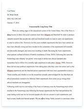
1.Generate a scatterplot for SALES vs. CALLS, including the graph of the “best fit” line.
Interpret.

After interpreting the scatter plot, it is evident that the slope of the ‘best fit’ line is positive, which indicates that sales amount varies directly with calls. As call increases, the sales amount increases as well.

2.Determine the equation of the “best fit” line, which describes the relationship between
SALES and CALLS.
The equation of the ‘best fit’ line or the regression equation is SALES(Y) = 9.638 + 0.2018 CALLS(X1)

3.Determine the coefficient of correlation. Interpret:
MINTAB Results:
Correlations: SALES(Y), CALLS(X1)

Pearson correlation of SALES(Y) and CALLS(X1) = 0.871
P-Value = 0.000

The coefficient of correlation is 0.871. The correlation coefficient is positive so this indicates a positive or direct relationship between the variables. The correlation coefficient is far from the P-Value of 0.000. This means that there is an extremely low chance that Sales and Calls results are wrong and we can be confident in interpretation.

4.Determine the coefficient of determination. Interpret.
MINTAB Results:

S = 2.05708 R-Sq = 75.9% R-Sq(adj) = 75.7%

The index of determination is the r-square = 0.759. The coefficient of determination is a key output of regression analysis. It is interpreted as the proportion of the variance in the dependent variable that is predictable from the independent variable, which for this regression model is 75.9%.

5.Test the utility of this regression model (use a two tail test with α =.05).
Interpret your results, including the p-value.
MINTAB Results:
Coefficients:

Term Coef SE Coef T P 95% CI
Constant 9.63795 1.87156 5.1497 0.000 (5.92391, 13.3520) CALLS(X1) 0.20175 0.01148 17.5797 0.000 (0.17898, 0.2245)

Since the significance level is α = 0.05 and we know that if the p-value is less than or equal to the level of significance we reject the null hypothesis because the test statistic falls in the rejection region. The p-value 0.000 is less than 0.05 so we will reject the null hypothesis and accepting the alternative hypothesis and there is no significant correlation and in conclusion the overall test of significance, the regression model is valid.

6.Based on your findings in 1-5, what is your opinion about using CALLS to predict SALES? Explain. After analysing scatterplot for SALES vs. CALLS, calls is a great predictor of sales. As calls increase the sales increases and they are correlated. Therefore, as the calls in the call center increase, the company makes more money. 7.Compute the 95% confidence interval for beta-1 (the population slope).

Interpret this interval.
The 95% confidence interval for β1 is given as (0.17898, 0.2245). The value of the slope of the regression line is expected to lie within the interval (0.17898, 0.2245) about 95% of the time. 8.Using an interval, estimate the average weekly sales for weekly calls that are 150.

Interpret this interval.
MINTAB Results:
Predicted Values for New Observations:

New Obs Fit SE Fit 95% CI 95% PI 1 39.9008 0.248127 (39.4084, 40.3932) (35.7890, 44.0126)

Values of Predictors for New Observations

New Obs CALLS(X1)
1 150
The average weekly sales for weekly calls that are 150 is expected to lie within the interval (39.4084, 40.3932). This is the 95% confidence interval estimate of sales for an average weekly calls of 150. 9.Using an interval, predict the weekly sales when weekly calls that are 150.

Interpret this interval.
The predicted weekly sales, when weekly calls are 150 is expected to lie within the interval (35.7890, 44.0126). This is the 95% prediction estimate of sales for weekly calls of 150. 10.What can we say about the weekly sales when weekly calls are 300.

Explain your answer.
MINTAB Results:
Descriptive Statistics: SALES(Y), CALLS(X1)

Variable N Mean SE Mean StDev Minimum Median Maximum SALES(Y) 100 42.340 0.417 4.171 32.000 42.000 52.000 CALLS(X1) 100 162.09 1.80 18.01 124.00 160.50 201.00

Since the maximum value of the predictor variable (calls) is used to formulate the given regression model is 201.00, which is less than 300, we cannot use the given regression model to accurately estimate the weekly sales for weekly call of 300. So we can’t say anything about the weekly sales when weekly calls are 300. In an attempt to improve this model, we attempt to do a multiple regression model predicting SALES based on CALLS, TIME, and YEARS.

11.Using MINITAB run the multiple regression analysis using the variables CALLS, TIME, and YEARS to predict SALES. State the equation for this multiple regression model. MINTAB Results:
General Regression Analysis: SALES(Y) versus CALLS(X1), TIME(X2), YEARS(X3): Regression Equation
SALES(Y) = 8.60864 + 0.20551 CALLS(X1) + 0.0520391 TIME(X2) – 0.181791 YEARS(X3)
Coefficients

Term Coef SE Coef T P 95% CI
Constant 8.60864 3.55193 2.4236 0.017 ( 1.55811, 15.6592) CALLS(X1) 0.20551 0.01409 14.5811 0.000 ( 0.17753, 0.2335) TIME(X2) 0.05204 0.10570 0.4923 0.624 (-0.15778, 0.2619) YEARS(X3) -0.18179 0.16932 -1.0736 0.286 (-0.51789, 0.1543)

Summary of Model

S = 2.06152 R-Sq = 76.31% R-Sq(adj) = 75.57%
PRESS = 442.906 R-Sq(pred) = 74.29%

Analysis of Variance

Source DF Seq SS Adj SS Adj MS F P Regression 3 1314.45 1314.45 438.151 103.097 0.000000 CALLS(X1) 1 1307.75 903.56 903.561 212.609 0.000000 TIME(X2) 1 1.81 1.03 1.030 0.242 0.623624 YEARS(X3) 1 4.90 4.90 4.899 1.153
0.285676 Error 96 407.99 407.99 4.250

Total 99 1722.44

The multiple regression equation is:
SALES(Y) = 8.60864 + 0.20551 CALLS(X1) + 0.0520391 TIME(X2) – 0.181791 YEARS(X3)

12.Perform the Global Test for Utility (F-Test). Explain your conclusion.

The p-value (0.000) is less than 0.05. So, we reject the null hypothesis that there is no significant correlation and conclude that, according to the overall test of significance, the multiple regression model is valid.

13.Perform the t-test on each independent variable. Explain your conclusions and clearly state how you should proceed. In particular, which independent variables should we keep and which should be discarded. MINTAB Results:

Coefficients:

Term Coef SE Coef T P 95% CI
Constant 8.60864 3.55193 2.4236 0.017 ( 1.55811, 15.6592) CALLS(X1) 0.20551 0.01409 14.5811 0.000 ( 0.17753, 0.2335) TIME(X2) 0.05204 0.10570 0.4923 0.624 (-0.15778, 0.2619) YEARS(X3) -0.18179 0.16932 -1.0736 0.286 (-0.51789, 0.1543)

MINTAB Results:
Coefficients:

Term Coef SE Coef T P 95% CI
Constant 10.0815 1.90699 5.2866 0.000 ( 6.29669, 13.8664) CALLS(X1) 0.2015 0.01146 17.5856 0.000 ( 0.17876, 0.2242) YEARS(X3) -0.1937 0.16694 -1.1601 0.249 (-0.52499, 0.1377)

The independent variables CALLS and YEARS should be kept because there is a significant contribution in the regression model. The variable of TIME should be discarded because it does not have a significant contribution in the regression model. 14.Is this multiple regression model better than the linear model that we generated in parts 1-10? Explain. Regression Analysis: SALES(Y) versus CALLS(X1)

The regression equation is

SALES(Y) = 9.638 + 0.2018 CALLS(X1)

S = 2.05708 R-Sq = 75.9% R-Sq(adj) = 75.7%

General Regression Analysis: SALES(Y) versus CALLS(X1), YEARS(X3) Regression Equation

SALES(Y) = 10.0815 + 0.201501 CALLS(X1) – 0.193667 YEARS(X3)

Summary of Model

S = 2.05346 R-Sq = 76.25% R-Sq(adj) = 75.76%
PRESS = 435.101 R-Sq(pred) = 74.74%

The higher the value of r-square, the better is the regression model. The value of r-square(adj) is slightly less for the multiple regression model of a 76% (75.76) as compared to that of r-square of the linear regression model which is about 76%(75.9) and so the linear regression model is slightly better than the multiple regression model.