Audio Watermarking

1. INTRODUCTION

With the rapid development of the speech, audio, image, and video compression methods, currently it is not a difficult task to spread digital multimedia over Internet. This makes the protections of digital intellectual property rights and content authentications have been a serious problem. Hence the technology of digital watermarking is received a large deal of attention. Generally, digital watermarking techniques are based on either spread spectrum methods or changing the least significant bits of selected coefficients of a certain signal transform. For speech watermarking, to ensure the embedded watermark is imperceptible, the audio marking phenomenon is considered together with these conventional techniques.

In addition, a speech watermarking system should be robust to various speech compression operations. The development of speech watermarking algorithms, therefore, involves a trade-off among speech fidelity, robustness, and watermark pattern embedding rate specifications. The speech watermarking techniques usually embed speech watermark in unnecessary parts of speech signal, or in human insensitivity auditory regions. Some of speech watermarking methods will change an interval to embed watermark. However, this kind of method has a drawback that is the unavoidably degradation of robustness.

In the other methods, the watermarks are embedded by the use of counterfeit human speech. It is unfortunate that such type of method also has the defect of weak robustness especially when the counterfeit human speech is destroyed. The distortion of the counterfeit human speech will also lead to the damage of the watermark

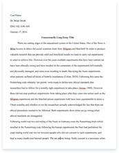
Fig 1.1: Block of General watermarking Scheme

Therefore, we can define watermarking systems as systems in which the hidden message is related to the host signal and non-watermarking systems in which the message is unrelated to the host signal. On the other hand, systems for embedding messages into host signals can be divided into steganographic systems, in which the existence of the message is kept secret, and non-steganographic systems, in which the presence of the embedded message does not have to be secret.

Audio watermarking algorithms are characterized by five essential properties, namely perceptual transparency, watermark bit rate, robustness, blind/informed watermark detection, and security

Perceptual transparency

In most of the applications, the watermark-embedding algorithm has to insert additional data without affecting the perceptual quality of the audio host signal. The fidelity of the watermarking algorithm is usually defined as a perceptual similarity between the original and watermarked audio sequence. However, the quality of the watermarked audio is usually degraded, either intentionally by an adversary or unintentionally in the transmission process, before a person perceives it. In that case, it is more adequate to define the fidelity of a watermarking algorithm as a perceptual similarity between the watermarked audio and the original host audio at the point at which they are presented to a consumer.

Watermark bit rate

The bit rate of the embedded watermark is the number of the embedded bits within a unit of time and is usually given in bits per second (bps). Some audio watermarking applications, such as copy control, require the insertion of a serial number or author ID, with the average bit rate of up to 0.5 bps. For a broadcast monitoring watermark, the bit rate is higher, caused by the necessity of the embedding of an ID signature of a commercial within the first second at the start of the broadcast clip, with an average bit rate up to 15 bps. In some envisioned applications, e.g. hiding speech in audio or compressed audio stream in audio, algorithms have to be able to embed watermarks with the bit rate that is a significant fraction of the host audio bit rate, up to 150 kbps.

Robustness

The robustness of the algorithm is defined as an ability of the watermark detector to extract the embedded watermark after common signal processing manipulations. A detailed overview of robustness tests is given in Chapter 3. Applications usually require robustness in the presence of a predefined set of signal processing modifications, so that watermark can be reliably extracted at the detection side. For example, in radio broadcast monitoring, embedded watermark need only to survive distortions caused by the transmission process, including dynamic compression and low pass filtering, because the watermark detection is done directly from the broadcast signal. On the other hand, in some algorithms robustness is completely undesirable and those algorithms are labeled fragile audio watermarking algorithms.

Blind or informed watermark detection

In some applications, a detection algorithm may use the original host audio to extract watermark from the watermarked audio sequence (informed detection). It often significantly improves the detector performance, in that the original audio can be subtracted from the watermarked copy, resulting in the watermark sequence alone. However, if detection algorithm does not have access to the original audio (blind detection) and this inability substantially decreases the amount of data that can be hidden in the host signal. The complete process of embedding and extracting of the watermark is modeled as a communications channel where watermark is distorted due to the presence of strong interference and channel effects. A strong interference is caused by the presence of the host audio, and channel effects correspond to signal processing operations.

Security

Watermark algorithm must be secure in the sense that an adversary must not be able to detect the presence of embedded data, let alone remove the embedded data. The security of watermark process is interpreted in the same way as the security of encryption techniques and it cannot be broken unless the authorized user has access to a secret key that controls watermark embedding. An unauthorized user should be unable to extract the data in a reasonable amount of time even if he knows that the host signal contains a watermark and is familiar with the exact watermark embedding algorithm. Security requirements vary with application and the most stringent are in cover communications applications, and, in some cases, data is encrypted prior to embedding into host audio.

Theory:-

The fundamental process in each watermarking system can be modeled as a form of communication where a message is transmitted from watermark embedder to the watermark receiver. The process of watermarking is viewed as a transmission channel through which the watermark message is being sent, with the host signal being a part of that channel. In Figure 2, a general mapping of a watermarking system into a communications model is given. After the watermark is embedded, the watermarked work is usually distorted after watermark attacks. The distortions of the watermarked signal are, similarly to the data communications model, modeled as additive noise.

Fig 1.2: Basic Watermarking system equivalent to a communication system

In this project, signal processing methods are used for watermark embedding and extracting processes, derivation of perceptual thresholds, transforms of signals to different signal domains (e.g. Fourier domain, wavelet domain), filtering and spectral analysis. Communication principles and models are used for channel noise modeling, different ways of signaling the watermark (e.g. a direct sequence spread spectrum method, frequency hopping method) derivation of optimized detection method (e.g. matched filtering) and evaluation of overall detection performance of the algorithm (bit error rate, normalized correlation value at detection). The basic information theory principles are used for the calculation of the perceptual entropy of an audio sequence, channel capacity limits of a watermark channel and during design of an optimal channel coding method.

During transmission and reception signals are often corrupted by noise, which can cause severe problems for downstream processing and user perception. It is well known that to cancel the noise component present in the received signal using adaptive signal processing technique, a reference signal is needed, which is highly correlated to the noise. Since the noise gets added in the channel and is totally random, hence there is no means of creating a correlated noise, at the receiving end. Only way possible is to somehow extract the noise, from the received signal, itself, as only the received signal can say the story of the noise added to it. Therefore an automated means of removing the noise would be an invaluable first stage for many signal-processing tasks. Denoising has long been a focus of research and yet there always remains room for improvement.

Simple methods originally employed the use of time-domain filtering of the corrupted signal, however, this is only successful when removing high frequency noise from low frequency signals and does not provide satisfactory results under real world conditions. To improve performance, modern algorithms filter signals in some transform domain such as z for Fourier. Over the past two decades, a flurry of activity has involved the use of the wavelet transform after the community recognized the possibility that this could be used as a superior alternative to Fourier analysis. Numerous signal and image processing techniques have since been developed to leverage the power of wavelets. These techniques include the discrete wavelet transform, wavelet packet analysis, and most recently, the lifting scheme.

2. Speech Processing

Speech Production:-
Speech is produced when air is forced from the lungs through the vocal cords and along the vocal tract. The vocal tract extends from the opening in the vocal cords (called the glottis) to the mouth, and in an average man is about 17 cm long. It introduces short-term correlations (of the order of 1ms) into the speech signal, and can be thought of as a filter with broad resonances called formants. The frequencies of these
formants are controlled by varying the shape of the tract, for example by moving the position of the tongue. An important part of many speech codec is the modeling of the vocal tract as a short-term filter. As the shape of the vocal tract varies relatively slowly, the transfer function of its modeling filter needs to be updated only relatively infrequently (typically every 20 ms or so).

From the technical, signal-oriented point of view, the production of speech is widely described as a two-level process. In the first stage the sound is initiated and in the second stage it is filtered on the second level. This distinction between phases has its origin in the source-filter model of speech production.

Fig 3: Source Filter Model of Speech Production

The basic assumption of the model is that the source signal produced at the glottal level is linearly filtered through the vocal tract. The resulting sound is emitted to the surrounding air through radiation loading (lips). The model assumes that source and filter are independent of each other. Although recent findings show some interaction between the vocal tract and a glottal source (Rothenberg 1981; Fant 1986), Fant’s theory of speech production is still used as a framework for the description of the human voice, especially as far as the articulation of vowels is concerned.

Speech Processing:-
The term speech processing basically refers to the scientific discipline concerning the analysis and processing of speech signals in order to achieve the best benefit in various practical scenarios. The field of speech processing is, at present, undergoing a rapid growth in terms of both performance and applications. The advances being made in the field of microelectronics, computation and algorithm design stimulate this. Nevertheless, speech processing still covers an extremely broad area, which relates to the following three engineering applications:

• Speech Coding and transmission that is mainly concerned with man-to man voice communication. • Speech Synthesis which deals with machine-to-man communications. • Speech Recognition relating to man-to machine communication.

Speech Coding:-
Speech coding or compression is the field concerned with compact digital representations of speech signals for the purpose of efficient transmission or storage. The central objective is to represent a signal with a minimum number of bits while maintaining perceptual quality. Current applications for speech and audio coding algorithms include cellular and personal communications networks (PCNs), teleconferencing, desktop multi-media systems, and secure communications.

The Discrete Wavelet Transform:-
The Discrete Wavelet Transform (DWT) involves choosing scales and positions based on powers of two’s, So called dyadic scales and positions. The mother wavelet is rescaled or dilated by powers of two and translated by integers. Specifically, a function f(t) L2(R) (defines space of square integral functions) can be represented as

(3.4)

The function ψ(t) is known as the mother wavelet, while φ(t) is known as the scaling Function. The set of functions

Where Z is the set of integers is an ortho- normal basis for L2(R). The numbers a(L, k) are known as the approximation coefficients at scale L, while d(j, k) are known as the detail coefficients at scale j.

The approximation and detail coefficients can be expressed as:

To provide some understanding of the above coefficients consider a projection fl(t) of the function f(t) that provides the best approximation (in the sense of minimum error energy) to f(t) at a scale l. This projection can be constructed from the coefficients a(L, k), using the equation (3.5)

As the scale l decreases, the approximation becomes finer, converging to f(t) as l → 0. The difference between the approximation at scale l + 1 and that at l, fl+1(t) – fl(t), is Completely described by the coefficients d(j, k) using the equation

(3.6)

Using these relations, given a(L, k) and {d(j, k) | j ≤ L}, it is clear that we can build the approximation at any scale. Hence, the wavelet transform breaks the signal up into a coarse approximation fL(t) (given a(L, k)) and a number of layers of detail {fj+1(t)-fj(t)| j < L} (given by {d(j, k) | j ≤ L}). As each layer of detail is added, the approximation at the next finer scale is achieved.

Vanishing Moments
The number of vanishing moments of a wavelet indicates the smoothness of the wavelet function as well as the flatness of the frequency response of the wavelet filters (filters used to compute the DWT).Typically a wavelet with p vanishing moments satisfies the following equation or equivalently.

For the representation of smooth signals, a higher number of vanishing moments leads to a faster decay rate of wavelet coefficients. Thus, wavelets with a high number of vanishing moments lead to a more compact signal representation and are hence useful in coding
applications. However, in general, the length of the filters increases with the number of vanishing moments and the complexity of computing the DWT coefficients increases with the size of the wavelet filters.

The Fast Wavelet Transform Algorithm
The Discrete Wavelet Transform (DWT) coefficients can be computed by using Mallat’s Fast Wavelet Transform algorithm. This algorithm is sometimes referred to as the two-channel sub-band coder and involves filtering the input signal based on the wavelet function used. Implementation Using Filters To explain the implementation of the Fast Wavelet Transform algorithm consider the following equations:

(3.9)
The first equation is known as the twin-scale relation (or the dilation equation) and defines the scaling function φ. The next equation expresses the wavelet ψ in terms of the scaling function φ. The third equation is the condition required for the wavelet to be Orthogonal to the scaling function and its translates

The coefficients c(k) or {c0, .., c2N-1} in the above equations represent the impulse response coefficients for a low pass filter of length 2N, with a sum of 1 and a norm of1/2 The high pass filter is obtained from the low pass filter using the relationship g ( )k c( k ) k = −1 1− , where k varies over the range (1 . (2N . 1)) to 1.

Equation 2.7 shows that the scaling function is essentially a low pass filter and is used to define the approximations. The wavelet function defined by equation 2.8 is a high pass filter and defines the details. Starting with a discrete input signal vector s, the first stage of the FWT algorithm decomposes the signal into two sets of coefficients. These are the approximation coefficients cA1 (low frequency information) and the detail coefficients cD1 (high frequency information), as shown in the figure below.

Fig 3.3: Block diagram of DWT

The coefficient vectors are obtained by convolving s with the low-pass filter Lo_D for Approximation and with the high-pass filter Hi_D for details. This filtering operation is Then followed by dyadic decimation or down sampling by a factor of 2. Mathematically the two-channel filtering of the discrete signal s is represented by the expressions:

(3.10)

These equations implement a convolution plus down sampling by a factor 2 and give the forward fast wavelet transform. If the length of each filter is equal to 2N and the length of the original signal s is equal to n, then the corresponding lengths of the coefficients cA1 and cD1 are given by the formula:

(3.11)

This shows that the total length of the wavelet coefficients is always slightly greater than the length of the original signal due to the filtering process used.

Multilevel Decomposition
The decomposition process can be iterated, with successive approximations being decomposed in turn, so that one signal is broken down into many lower resolution Components. This is called the wavelet decomposition tree.

Fig 3.4: Wavelet decomposition tree
The wavelet decomposition of the signal s analysed at level j has the following structure [cAj, cDj, …, cD1].
Looking at a signals wavelet decomposition tree can reveal valuable information.

Since the analysis process is iterative, in theory it can be continued indefinitely. In reality, the decomposition can only proceed until the vector consists of a single sample. Normally, however there is little or no advantage gained in decomposing a signal beyond a certain level. The selection of the optimal decomposition level in the hierarchy depends on the nature of the signal being analysed or some other suitable criterion, such as the low-pass filter cut-off.

Signal Reconstruction

The original signal can be reconstructed or synthesised using the inverse discrete wavelet transform (IDWT). The synthesis starts with the approximation and detail coefficients cAj and cDj, and then reconstructs cAj-1 by up sampling and filtering with the reconstruction filters.

Fig 3.5: Block diagram of IDWT

The reconstruction filters are designed in such a way to cancel out the effects of aliasing introduced in the wavelet decomposition phase. The reconstruction filters (Lo_R and Hi_R) together with the low and high pass decomposition filters, forms a system known as quadrature mirror filters (QMF).

Methodology:

Speech water marking:
The speech water marking means embed a digital data(speech) into the other speech signal (.wav) or remove the signal components of desired signal is called speech water marking Here I have consider two speech signal like

1) Select the desired speech signal(.wav),read desired wave length and play the selected desired speech signal

2) Select the embedded speech signal (.wav), read and play the selected embedded speech signal

3) Select the desired speech signal (.wav), read selected desired speech signal

4) Than above signals applied discrete wave let transform with name of the wavelet “Haar” .Because we need required desired processing

5) Due to speech water marking: the desired signals one by one processing continues

Here I have used cat function.

6) Here water marking results playing

7) SWPR: stand for speech water marking signal play, due to recording

8) SWRP: stand for speech water marking signal recorded and playing